

Ocean/Sea Ice: Assimilation Setup: SLA
 The SLA observations used in GEOS ODAS5.2 (A004) are along-track merged products obtained from AVISO, referenced to a 7-year mean (January 1993 to January 1999). Because of the high resolution of the AVISO product (adjacent SLA measurements are approximately 20 km apart), the along-track observations are high-pass filtered using a Gaussian kernel with a stencil size of 21 and a decorrelation length scale of 100 km. The along-track variability over 200 km segments is used as a proxy for the errors of representativeness; a snapshot of that estimate is depicted in Figure 4. No instrument error is imposed. 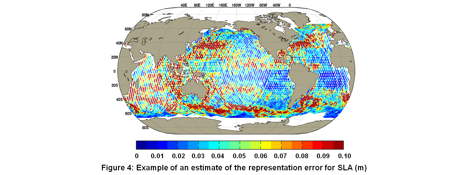 The model SLA is given by η′ = η-n̄, where the mean sea level n̄, also referred to as the mean dynamic topography (MDT), is the 7-year mean sea level of GEOS ODAS5.1 (A005) from January 1993 to December 1999 (see Figure 5) and η is the total sea level from the barotropic component of the ocean model. 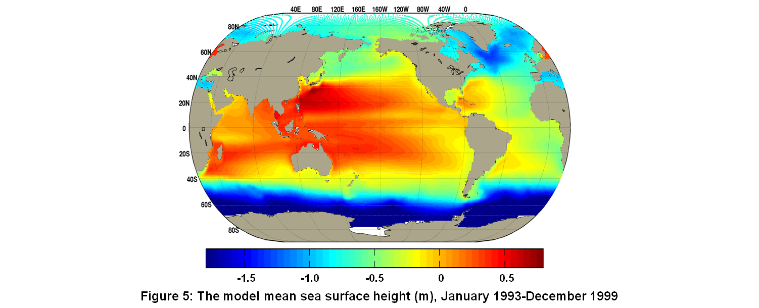 Within the EnOI framework used for the assimilation of the SLA, an increment in η is accompanied by an increment in the three-dimensional T field (see last column of line 3 of Table 1). A poor estimate of the T could be caused by the wrong choice of MDT (n̄) or wrong cross-covariances between SLA and T. Whether the MDT chosen in the analysis is appropriate is still an active area of research in the community and will not be discussed in this report. In order to separate the two sources of error, and only investigate the robustness of the cross-covariances, an objective (model-less) analysis was carried out, in which SLA are used as a predictor for T anomalies (hereafter, T′) over the entire water column, therefore avoiding the need for an estimate of the MDT. To simplify the vertical projection, the daily gridded SLA from AVISO is used. Further, we assume that the errors are horizontally uncorrelated, an observation of SLA at (x,y) is only influencing a single water column of T′(z) at (x,y). Using this simplification, the problem of estimating the three-dimensional T′ reduces to many independent one-dimensional vertical projections (as many as there are observations). For this purpose, the entire set of EOFs are used (286) for the computation of the covariance between η and T′(z) at location x,y. Because of the relatively large size of the ensemble, localization of the vertically dependent covariance is not necessary. |