

Ocean/Sea Ice: Assimilation Method
Data assimilation refers to optimization methods that seek the true state of a system by optimally
combining observations with a physical representation of that system. For all methods used in this
report, the analysis can be expressed as a linear regression in observation space:
 where 𝒙𝒂 is the analysis, 𝒙𝒇 is the forecast or prior state, the ri are covariances between the state and the observations, also referred to as the representers (Kimeldorf and Wahba 1970; Bennett 1992), No is the number of observations and the βi are the representer coefficients. The βi are determined by solving linear system  where H is a linear observation operator, the i-th column of 𝑷𝑯𝑻 is the i-th representer ri, y is the vector containing the No observations, R is an observation error-covariance matrix, and h is the model-data misfit. The iODAS is a sequential ensemble assimilation software system that includes a wide range of algorithm implementations, from simple optimal interpolation (OI: Eliassen 1954) to more expensive ensemble methods such as ensemble Kalman filtering or particle filtering. The reanalysis for the seasonal forecast initialization use the ensemble optimal interpolation (e.g., Oke et al. 2010, Wan et al. 2010) implementation where the time dependency of the covariances is neglected and P is estimated from the statistics of model run histories or from combinations of model histories. EnOI methods are often competitive with the EnKF because they make up for the performance degradation due to neglecting the forecast-error evolution by computing their statistics from a much larger ensemble. Keppenne et al. (2013) introduces an additional approach to estimating the background error covariances the spatial approximation of forecast errors (SAFE) technique. This approach is used in the GEOS ODAS for the assimilation of surface observations such as SST and sea surface salinity (SSS) (see Table 1 below). 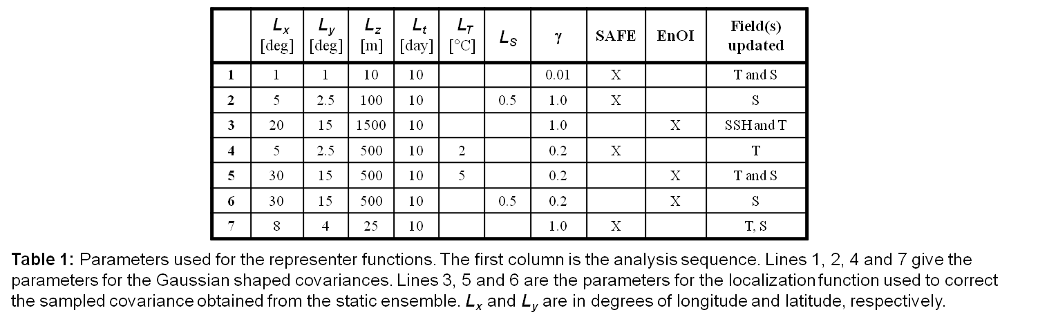 Covariance Modeling and LocalizationIn the Optimal Interolation (OI) implementation, the covariances are assumed to have a Gaussian shape, approximated by the function given by as a special case of equation (1.0) of Gaspari and Cohn (1999). Dependencies on the background flow are obtained through the application of a localization function that uses Euclidean distance in T, S and density space. For example, a continuous form of the i-th representer can be written as follows,  where (xi,yi,zi,ti) is the space-time position of an observation, αi is an estimate of the background-error variance at the location of the observation, v is T, S or density, and Lx etc. are the vanishing-correlation length scales. The parameter λ is an inflation factor that is determined by  where γ is prescribed and represents the target ratio of background error standard deviation to observational error standard deviation and where ‖ ‖ represents the L2 vector norm. Finally, φ is a smooth,horizontally varying field that imposes the constraint that a representer does not cross major land boundaries; for example, a representer corresponding to an observation in the Gulf of Mexico will not influence the western Pacific. The SAFE implemenatation is similar to OI, except that the amplitude αi of the Gaussian covariances in (4.0) and cross-covariances are estimated from the model state itself. Unlike the SAFE or OI, the EnOI uses covariances estimated from an ensemble of model states. Spurious long-range covariances are filtered using localization in space, while dependencies on the background flow are obtained in the same manner as the OI method. The ocean and sea-ice analyses used in the seasonal forecast are from ODAS5.1 (A005) and ODAS5.2 (A004). |