

Perturbations
|
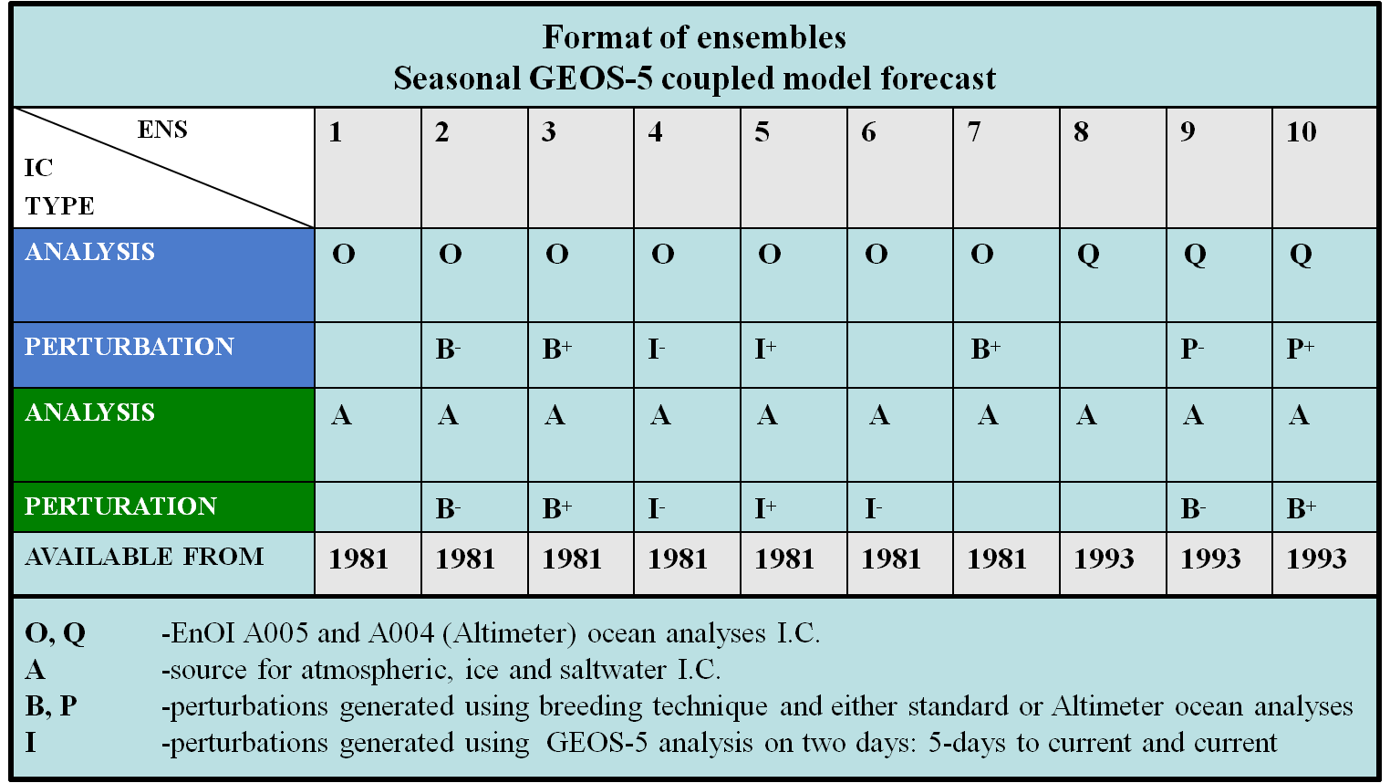
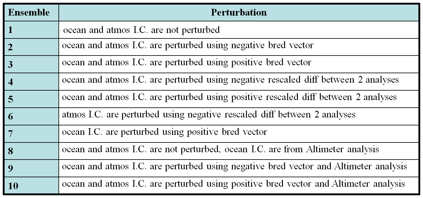
Ensembles of numerical forecasts based on perturbed initial conditions have long been used to improve estimates of both weather and climate forecasts. GEOS-5 seasonal forecast is arranged so that it uses a set of 10 ensembles for the forecast initialized on the day closest to the beginning of the month, and one ensemble otherwise. Initial perturbation method, that adds small perturbation to analysis initial conditions, is used to generate the ensemble forecast. Since one goal has been the use of the ensemble spread as an indicator of expected forecast skill, bred vectors [Toth and Kalnay, 1993] have been used as perturbations to capture the fastest growing modes on weather time scales. More recently, the coupled breeding method was developed for coupled atmosphere ocean systems to capture the dominant mode of coupled instabilities associated with the El Niño/Southern Oscillation (ENSO) [Cai et al., 2003; Yang et al., 2006, 2008; Ham et al., 2012].
The breeding is applied from 1980 with the aim of capturing the fastest-growing errors in the seasonal forecasts. Two-sided breeding is applied, which means positive and negative bred runs are restarted every month by adding and subtracting the bred vector to the initial conditions generated from the Ensemble Optimal Interpolation (EnOI) option of the GEOS ocean data assimilation system, forced with NASA’s Modern-Era Retrospective analysis for Research and Applications (MERRA) [Rienecker et al., 2011]. The rescaling interval chosen for the breeding is one month. The rescaling norm is the RMS difference of the instantaneous sea surface temperatures (SSTs) from the positive and negative bred runs; the region for defining the norm is the tropical Pacific domain over 120E-90W, and 10S-10N. At every re-initialization during the breeding cycle, perturbations are re-scaled so that the magnitude of the norm is reduced to 10% of the natural variability of SST over the norm region (i.e. 0.48_ C). Another method to perturb initial conditions is based on GEOS-5 analysis on two different days. Similar to breeding, the perturbations are re-scaled and the magnitude of the norm reduced to 10% of the natural variability of SST over the norm region (i.e. 0.48_ C). Combination of these 2 methods is used in generating the ensembles for seasonal forecast. Yoo-Geun Ham, Michele M. Rienecker, Siegfried Schubert, Jelena Marshak, Sang-Wook Yeh, and Shu-Chih Yang, 2012: The Decadal Modulation of Coupled Bred Vectors. GEOPHYSICAL RESEARCH LETTERS, VOL. 39, L20712, doi: 10.1029/2012GL053719 |
|
|
The following variables are perturbed: On ocean model grid - temperature and salinity (ocean_temp_salt.res.nc), ocean velocities (ocean_velocity.res.nc), surface temperature, salinity and velocities, sea level and frazil (ocean_sbc.res.nc), ice velocity and strain rate components, ice strength, extent and stress tensor components (first 18 variables from seaice_internal_rst. On atmospheric grid - wind components, potential temperature, surface pressure (rst fvcore_internal) and specific humidity (moist_internal_rst). On tiles - skin temperature, salinity and depth (first seven variables from saltwater_internal_rst). |