

Ocean/Sea Ice: Assimilation Setup: T(z), S(z)
 The assimilation of in-situ profiles of temperature (T) and salinity (S) correspond to sequences 5 and 6 of Table 1. The observations are assimilated twice, in a multi-scale fashion, with the second assimilation being identical to the first except for the horizontal localization scales that are 50% of the scales used in the first assimilation. While both T and S analyses use the EnOI algorithm, only step 5, consisting of the analysis of T profiles, is multivariate (increments in T have corresponding increments in S). Step 6 consists of the univariate assimilation of S profiles. Since most S profiles have a corresponding T profile, salinity is not used to correct temperature. Prior to being assimilated, both T and S are binned according to the model’s levels and any profile that contains an observation that is six or more standard deviations (where the standard deviation is taken to be the standard deviation of the interannual variability) away from the WOA09 climatology is rejected. The observation error is modeled with an exponential decay written as,  where σi is the instrument error and the exponential decay term is a proxy for the errors of representation, parameterized with the e-folding depth scale z0=500 m and amplitude σ0. The parameters necessary to specify the observation error according to equation (6.0) are given in Table 3. 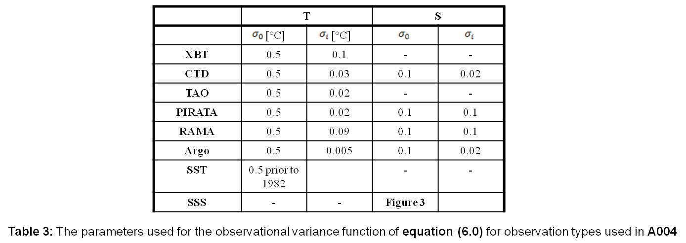 The covariances estimated from the static ensemble are localized using equation (4.0) and the parameterization given in lines 6 and 7 of Table 1. When assimilating T (or S), v in equation (4.0) is T (or S). This localization choice allows for small vertical scales above the thermocline, where the extent of vertical scales is mostly limited by the localization in T (S) and large scale below the thermocline where the vertical influence of the observation is limited by Lz. |