

Ozone extremes over the U.S. tracked by NASA’s composition forecasting system
In May, the Midwest U.S. experienced high levels of surface ozone that exceeded the National Ambient Air Quality Standard and posed a risk to millions of people and thousands of acres of crops. The region was already grappling with poor air quality caused by smoke drifting south from the massive fires in Alberta. Such regional ozone episodes occur almost every summer in different parts of the country, and accurate forecasts of such events can help mitigate their impact on human health and agriculture. The NASA Global Modeling and Assimilation Office (GMAO) operates the Goddard Earth Observing System (GEOS) Composition Forecasting (GEOS-CF; Keller et al., 2021) system that uses a detailed atmospheric chemistry model embedded in the GEOS model to provide global near real-time simulations and 5-day forecasts of surface ozone. Here we show that the system captures such extreme ozone anomalies over the contiguous US.
Surface ozone forms in reactions involving nitrogen oxides (NOx) and volatile organic compounds (VOC) in sunlight. Ozone concentrations peak between May and September in most of the U.S., because of ample sunlight and high temperatures, which accelerate the photochemical formation of ozone. Higher temperatures also lead to increased VOC emissions from vegetation and increased risk of fire emissions. The highest ozone concentrations generally occur in sunny and stagnant weather conditions caused by slow-moving high-pressure systems.
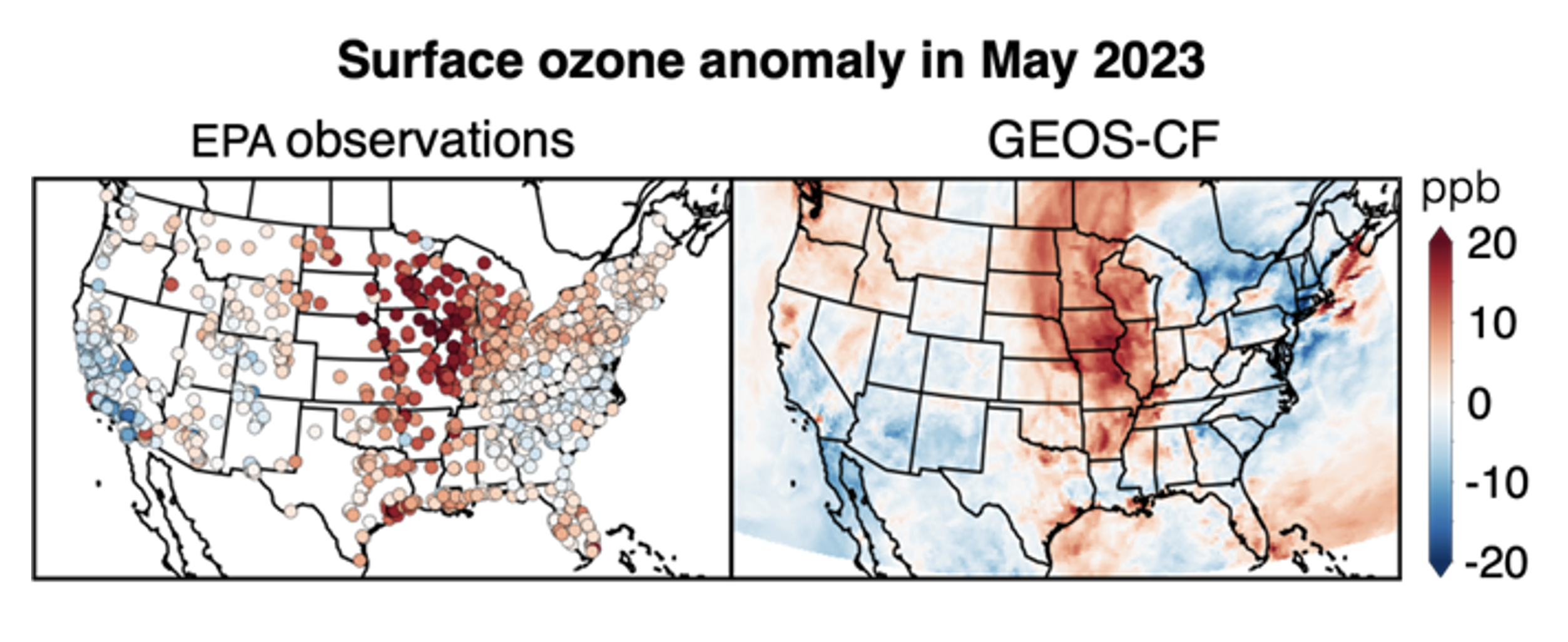
We begin by evaluating the near real-time GEOS-CF simulations for May 2023 using observations from the U.S. Environmental Protection Agency (EPA). Figure 1 shows the anomalies in the 90th percentile of the maximum daily 8-hour average (MDA8) ozone concentrations for May 2023 compared to the mean for May 2019-22 in the EPA observations and GEOS-CF. The EPA data show that ozone concentrations were 10-20 ppb higher this May compared to the past four years across an area extending from Arkansas to Wisconsin. GEOS-CF captures the spatial extent and temporal variability of the elevated ozone, but the anomalies are underestimated in the upper Midwest and there is a mismatch in the anomaly direction in Pennsylvania. Assimilation of tropospheric gas observations from satellites and surface networks in the GEOS-CF system in the future could improve the model performance.
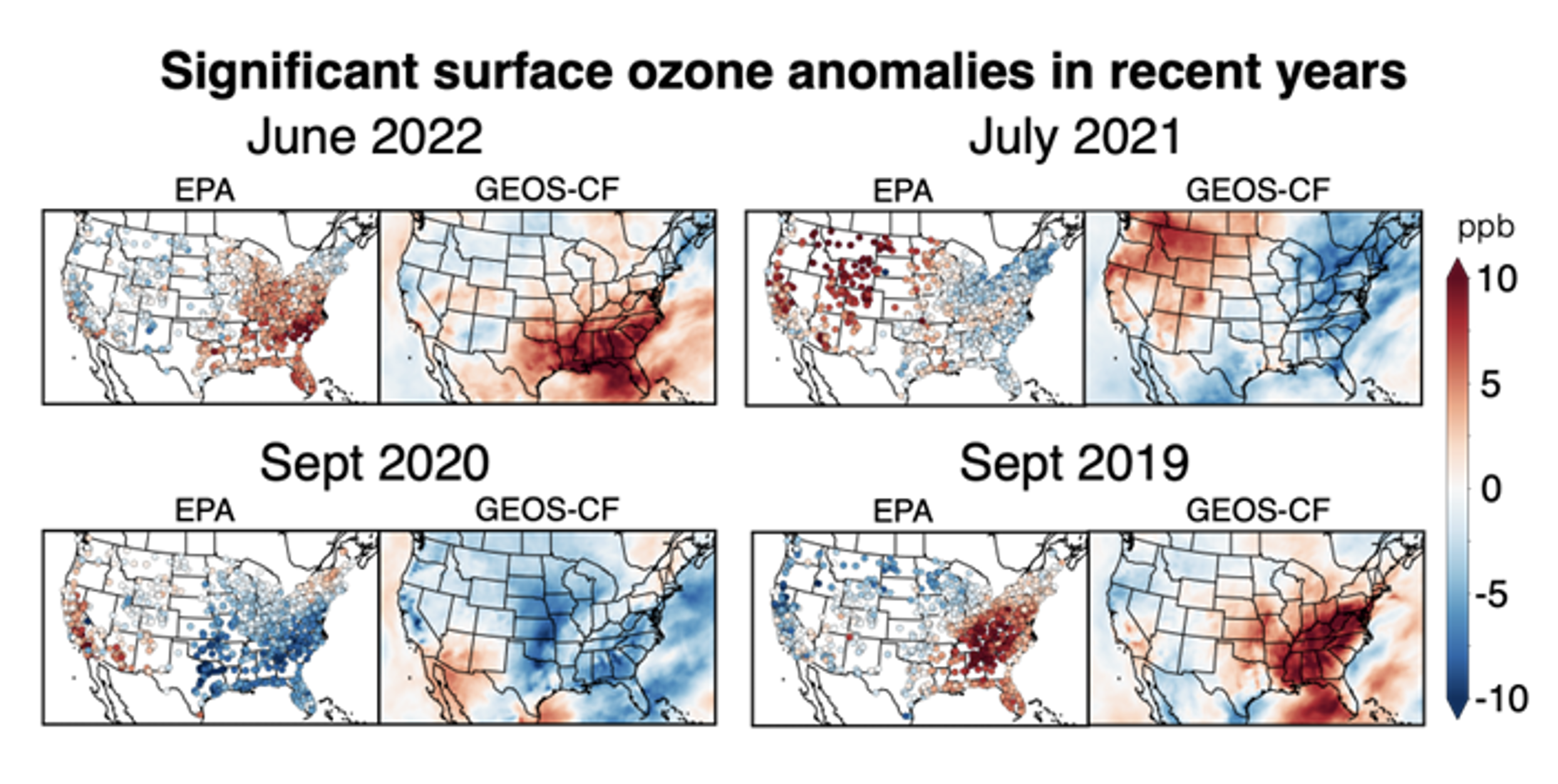
Extending the evaluation back to 2019, Figure 2 shows the observed and simulated ozone anomalies in the 90th percentile MDA8 ozone concentrations for selected summer months in 2019-22 when the anomalies were the largest and most widespread. The EPA observations show positive anomalies of more than 10 ppb over the eastern U.S. in June 2022 and September 2019 and over the western US in July 2021, and a negative anomaly of similar magnitude over the southeast US in Sept 2020. GEOS-CF reproduces the general location and direction of the observed anomalies but sometimes fails to simulate their magnitude. While GEOS-CF generally overestimates ozone concentrations over the eastern US in the summer (Keller et al., 2021), this analysis shows that the ozone anomalies in the model align better with the observed anomalies and can be used to identify anomalous ozone episodes, particularly over areas that are not covered by the EPA observations.
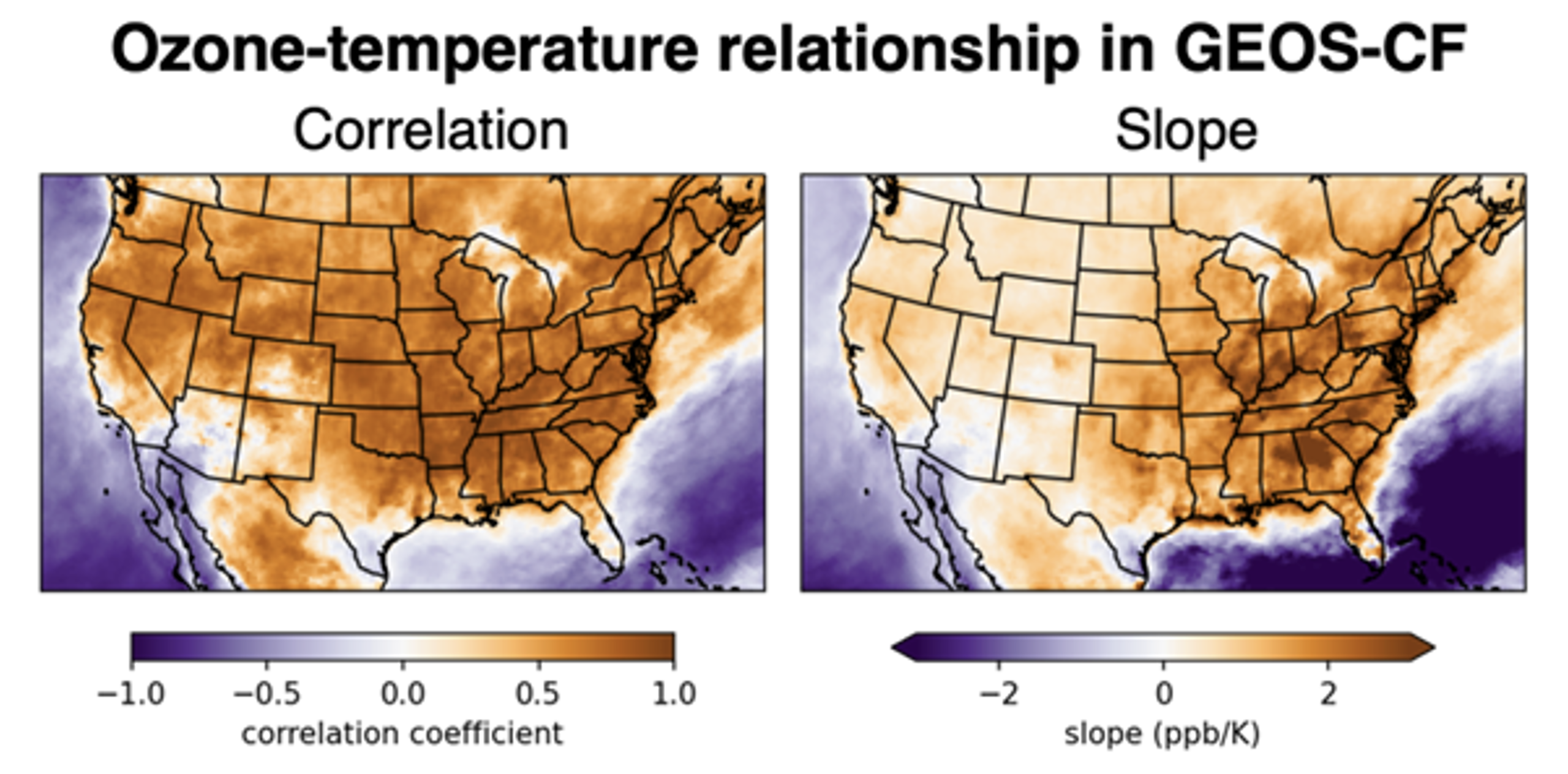
As surface ozone concentrations depend significantly on temperature, we examine the relationship between ozone and temperature in GEOS-CF. Figure 3 shows the correlation and the slope of the linear regression between the monthly 90th percentile MDA8 ozone and the 90th percentile daily maximum 10 m temperature in GEOS-CF for May-September, 2019-22. We see a high positive correlation between ozone and temperature across most of the U.S. There is a negative correlation over the oceans, where ozone is destroyed by photochemistry. The linear regression slope between ozone and temperature is more than 3 ppb per Kelvin in many areas of the eastern U.S., indicating a strong dependence of anomalies in ozone concentrations on temperature anomalies. The slopes are lower over the western US, where ozone production is not as significant. The strong relationship between ozone and temperature in the eastern U.S. could be utilized to statistically forecast ozone anomalies at seasonal timescales, leveraging the forecasts produced by the GMAO’s GEOS Sub-seasonal to Seasonal (GEOS-S2S) system.
References:
Keller, C. A., Knowland, K. E., Duncan, B. N., Liu, J., Anderson, D. C., Das, S., Lucchesi, R. A., Lundgren, E. W., Nicely, J. M., Nielsen, E., Ott, L. E., Saunders, E., Strode, S. A., Wales, P. A., Jacob, D. J., and Pawson, S.: Description of the NASA GEOS Composition Forecast Modeling System GEOS‐CF v1.0, J. Adv. Model. Earth Syst., 13, https://doi.org/10.1029/2020MS002413, 2021.