
An Analysis of Ocean, Land and Ice
The image demonstrates the capability of NASA’s Global Modeling and Assimilation Office (GMAO) to analyze the ocean, land, and ice surfaces using NASA’s satellite observations. Brightness temperatures from the Soil Moisture Active Passive (SMAP) mission and the Special Sensor Microwave Imager (SSM/I) are blended with model fields to derive salinity in the ocean, soil moisture at the land surface, and the thickness of sea ice.
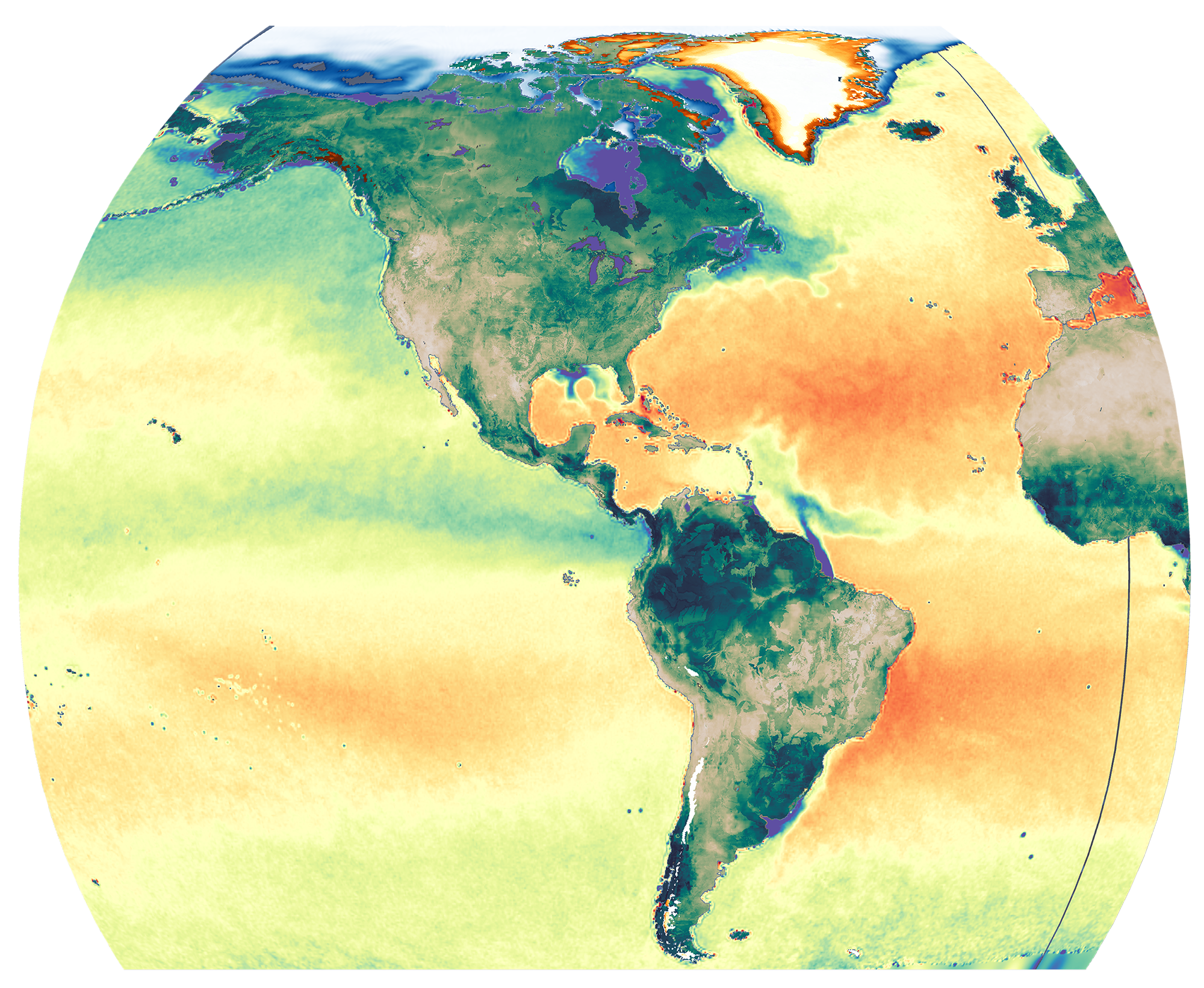
This image demonstrates the capability of NASA’s Global Modeling and Assimilation Office (GMAO) to analyze the ocean, land, and ice surfaces using NASA’s satellite observations. Brightness temperatures from the Soil Moisture Active Passive (SMAP) mission and the Special Sensor Microwave Imager (SSM/I) are blended with model fields to derive salinity in the ocean, soil moisture at the land surface, and the thickness of sea ice.
» Click for PDF «
Ocean: Monthly mean sea surface salinity (SSS) from SMAP satellite data
Satellite brightness temperature can be converted to salinity since the dielectric coefficient is a function of the salinity of sea water. These SSS data come from the processing of Meissner et al. (2019). Especially salty regions (red colors) can be seen at the center of the Atlantic gyres, where evaporation of water exceeds precipitation. In the south Atlantic along the coast of South America, the tight salinity gradient defines the northward flowing Malvinas (fresh, blue along the coast) and southward flowing Brazil currents (orange colors). In the North Atlantic, the Gulf Stream straddles the salinity gradient extending from the U.S. coast out into the Atlantic. The large freshwater outflow of the Mississippi leads to low salinity values in the Gulf of Mexico. Similarly, the freshwater outflow of the Amazon is evident, where it is first transported northwards along the coast by the North Brazil Current before it loops out into the Atlantic and is carried by the South Equatorial Counter-Current. The freshwater region that arises from strong rainfall in the Inter-Tropical Convergence Zone in the eastern Pacific is also clearly seen during August 2015, prior to the build-up of the big 2015 El Niño event.
Land: Mean soil wetness for August 2015 in the SMAP Level-4 soil moisture product
This quantity is derived by assimilating SMAP-observed brightness temperatures into the GMAO’s Catchment land surface model. Differences between the SMAP brightness temperatures and the model-derived estimates are used to update the model’s surface soil moisture, root-zone soil moisture and surface temperature states in order to create this assimilated dataset. This procedure implicitly interpolates the SMAP observations in space and time and enables the propagation of SMAP surface information to deeper soil layers. Deep green colors on the map clearly show areas that are climatologically very wet, including the Amazon rainforest, that experiences a large amount of precipitation, and the Hudson Plains peatlands in Canada, where a shallow water table and the high water retention of peat lead to wetter soil. The SMAP data also highlight weather-related variations. For example, in the U.S., the summer of 2015 brought extremely warm and dry conditions to the Southwest, the Southern Plains, and the Lower Mississippi, evident in the very dry soils in these areas (beige colors). The Midwest and Northeast US, on the other hand, experienced above average precipitation all summer, resulting in unusually wet soils there.
Cryosphere: Sea ice concentration and surface melt
Sea ice concentration during August 2015 derived from satellite brightness temperatures. Arctic sea ice concentrations can range from 100% (bright white colors) near the North Pole, to less than 15% (the typical threshold for calculating total ice extent) near Greenland and along the northern Canadian coast (blue colors). The data plotted here are from an optimal combination of two well-established methods (the NASA Team algorithm and NASA Bootstrap algorithm) for determining sea ice concentration from SSMIS (Special Sensor Microwave Imager/Sounder) and SSM/I on the Defense Meteorological Satellite Program’s DMAP-F8, F11 and F13 satellites.
Seasonal surface melting on glaciers and the Greenland Ice Sheet. The shading over these regions illustrates the intensity of melting, from white (no melt days) to dark orange, which indicates more than 120 days of surface melting. The gradient between intense and no melting is clear on the western margin of the Greenland Ice Sheet, while Alaskan glaciers, in particular, experienced intense, spatially extensive melting during this period. The data plotted are derived from a dynamical downscaling of the Modern-Era Retrospective analysis for Research and Applications, Version 2 (MERRA-2), GMAO’s most recent atmospheric reanalysis of the satellite era.