
General Characteristics of Stratospheric Singular Vectors
Ron Errico, Ron Gelaro, Elena Novakovskaia and Ricardo Todling
By studying mathematical models of the atmosphere, it is well known that if two earths existed at some instant of time with almost exactly the same weather patterns, those patterns would quickly become very different. This is one of the main reasons why weather forecasting is so difficult: we cannot predict the future accurately if we do not know the present perfectly. The earth's atmosphere and computer simulations of it are "unstable" with respect to small uncertainty in their specifications.
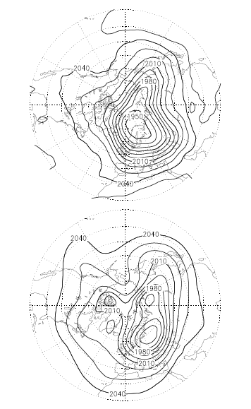
In this reported study, the instability of weather in the stratosphere is investigated. This is the first such study that uses a mathematical technique called "singular value decomposition," producing what are called "singular vectors" or "SVs" for short. These define the shapes of arbitrary changes to the weather patterns that will result in the largest change in the atmospheric evolution measured over some period of time. Unlike in earlier investigations of stratospheric instability, SV structures are allowed to change their shape with time, not only their magnitude and position.
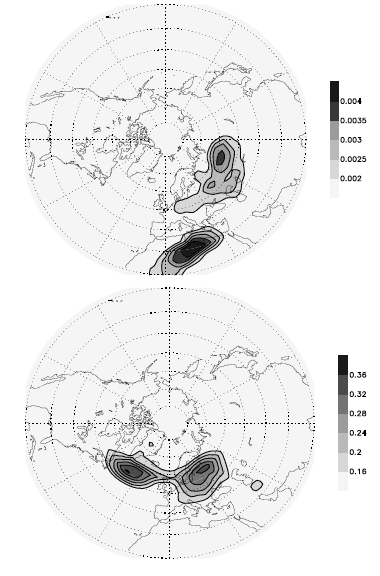
In this study, the basic properties of these stratospheric SVs are shown. Their precise determination is revealed to depend on how the evolved changes to the weather patterns are measured. For the most reasonable ways of measuring them, stratospheric SVs are shown to grow more slowly than their counterparts closer to the earth's surface. They also cover a much broader geographic region. They apparently grow in magnitude by optimally creating structures that, although initially distinct, evolve to strongly superimpose upon each other. In 5 days, they can become so large as to perhaps be able to account for the sudden changes in stratospheric weather patterns sometimes seen in the winter months.
(click on image to enlarge)
(click on image to enlarge)
Reference
Errico, R. M., R. Gelaro, E. Novakovskaia, and R. Todling, 2007: General Characteristics of Stratospheric Singular Vectors,Meteorol. Zeit. 16 (6), 685-692. (pdf)