Generalized Extreme Value (GEV) distribution: The GEV distribution is a family of continuous probability distributions developed within extreme value theory. Extreme value theory provides the statistical framework to make inferences about the probability of very rare or extreme events. The GEV distribution unites the Gumbel, Fréchet and Weibull distributions into a single family to allow a continuous range of possible shapes. These three distributions are also known as type I, II and III extreme value distributions. The GEV distribution is parameterized with a shape paramter, location parameter and scale parameter. The GEV Is equivalent to the type I, II and III, respectively, when a shape parameter is equal to 0, greater than 0, and lower than 0. Based on the extreme value theorem the GEV distribution is the limit distribution of properly normalized maxima of a sequence of independent and identically distributed random variables. Thus, the GEV distribution is used as an approximation to model the maxima of long (finite) sequences of random variables.
Equation: The cumulative distribution function (CDF) of the GEV distribution is
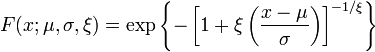 (1)
(1)
where three parameters, ξ, μ and σ represents a shape, location, and scale of the distribution function, respectively. Note that σ and 1 + ξ(x-μ)/σ must be greater than zero. The shape and location parameter can take on any real value.
The resulting probability distribution function (PDF) for two category of shape parameter (i.e., whether it is equal to zero or not) is
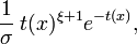
where
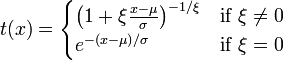 .
.
Further details on the three distributions and their examples are found at http://www.mathwave.com/articles/extreme-value-distributions.html
Application of GEV distribution (Return value calculation): Based on the extreme value theory that derives the GEV distribution, we can fit a sample of extremes to the GEV distribution to obtain the parameters that best explains the probability distribution of the extremes. In our present work, we first calculate daily maximum precipitation, the number of heavy rainfall events, the number of rainy days, and the consecutive dry days for each season over the last three decades. These extremes-related quantities are, respectively, fitted to the GEV distribution. From the fitted distribution, we can estimate how often the extreme quantiles occur with a certain return level. The return value is defined as a value that is expected to be equaled or exceeded on average once every interval of time (T) (with a probability of 1/T). Therefore, we obtain the equation, CDF of the GEV distribution (i.e., equation (1)) = 1-1/T. We call "T" on the right hand side of this equation as a return period, and "x" in equation (1) (left hand side) is the return value. The return value can be calculated by solving this equation (i.e., by inverting the GEV distribution). In our current work, We calculated return values for 2-, 5-, 10-, and 20-yr return period at each grid point.
References
European Climate Assessment & Dataset website (ECA&D): http://eca.knmi.nl.
Früh, B., H. Feldmann, H.-J. Panitz, and G. Schädler, D. Jacob, P. Lorenz, and K. Keuler, 2010: Determination of precipitation return values in complex terrain and their evaluation. J. Climate, 23, 2257-2274.
Rusticucci, M., and B. Tencer, 2008: Observed changes in return values of annual temperature extremes over Argentina. J. Climate, 21, 5455-5467.
Schubert, S. D., Y, Chang, M. J. Suarez, and P. J. Pegion, 2008: ENSO and wintertime extreme precipitation events over the contiguous United States. J. Climate, 21, 22-39.
Bonsal, B. R., X. Zhang, L. A. Vincent, and W. D. Hogg, 2001: Characteristics of daily and extreme temperatures over Canada. J. Climate, 14, 1959-1976.
Coles, S., 2001: An Introduction to Statistical Modeling of Extreme Values, Springer, 208pp.
Weiss, L. L., 1955: A nomogram based on the theory of extreme values for determining values for various return periods. Mon. Wea. Rev., 83, 69-71.